4 The Basic Formulas for Two-Dimensional Vectors

So, what about an equation to plug all the values into to solve for the resultant? It is absolutely a viable option and a path I personally prefer over a multitude of small calculations. The formula I have developed is as follows: the vector resultant in the 𝑥 and 𝑦 plane is equal to the 𝑥 component of the system squared plus the 𝑦 component of the system squared, all rooted.

[latex]{\vec{R}}_{xy}=\sqrt{\left(R_x\right)^2+\left(R_y\right)^2}[/latex]

Does it look familiar? Well, it should be no surprise that it resembles Pythagorean theorem. In a sense it is just Pythagorean theorem applied specifically. Chapter three summarized simply is this equation. But what does it mean? Why does it look so much like Pythagorean theorem?

It was not intended to look as such during its creation. While following the steps I took in my class notes to form this formula, I by chance stumbled upon the realization^[1] that vectors are just fancy trigonometry. I struggled with vectors beforehand, but after coming to this realization, I was able to fully excel within the field^[2]. We are utilizing the 𝑥 components and the 𝑦 components to solve for the resultant, also known as the hypotenuse. That said, we can combine the like terms of one or more vectors to solve for the resultant, specifically the 𝑥 and 𝑦 components of both vectors^[3]. This can be written as:

[latex]f_{1x}+f_{2x}=R_x[/latex]

and,

[latex]f_{1y}+f_{2y}=R_y[/latex]

When plugging into these values it is imperative to ensure that you maintain the calculated sign (whether that be positive or negative) as it will drastically change the system’s outcome entirely.

Allow me to explain; relative to the two equations above, if you have an [latex]f_{1x}[/latex] value of 20 units, and an [latex]f_{2x}[/latex] value of negative 10 units, your combined value, or your [latex]R_x[/latex] value, is 10 units as [latex]20+\left(-10\right)=10[/latex]. However, if you disregard the systems units you will end up with an incorrect value of 30 units simply due to the fact that you added the values rather than subtracting them.

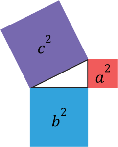
We then square root our [latex]R_x[/latex] and our [latex]R_y[/latex] values, because pythagorean theorem is secretly an area equation. Pythagorean theorem is [latex]a^2+b^2=c^2[/latex], this looks more familiar when broken down into its individual parts. Assume our [latex]a[/latex] value is two units, what do we get when we square this value? We get four units squared. Ring any bells?

These side lengths represent areas of squares, which when added give you a value of [latex]c[/latex], or our hypotenuse. It is not simply [latex]a^2+b^2=c^2[/latex], this equation is telling you that the area of square [latex]a[/latex] plus the area of square [latex]b[/latex] is equal to the area of square [latex]c[/latex]. This is why the rearranged equation is [latex]c=\sqrt{a^2+b^2}[/latex], because we have found our area of square [latex]c[/latex] by adding the areas of squares [latex]a[/latex] and [latex]b[/latex], we then need to take our area from square [latex]c[/latex] and square root it to get the side length of square [latex]c[/latex].

Our side lengths, also known as our [latex]f_x[/latex] and our [latex]f_y[/latex] values are calculated by basic trigonometry, sine, and cosine. It was determined that this was the most efficient method of determining our side lengths due to our given values of our hypotenuse and one of our angles. In a scenario that we have two vectors that we want to add together, the base equations look like this:

[latex]\left(cos\theta_{1xy}=\frac{f_{1x}}{\vec{f_1}}\right){\Rightarrow f}_{1x}[/latex]

[latex]\left(cos\theta_{2xy}=\frac{f_{2x}}{\vec{f_2}}\right)\Rightarrow f_{2x}[/latex]

[latex]\left(sin\theta_{1xy}=\frac{f_{1y}}{\vec{f_1}}\right)\Rightarrow f_{1y}[/latex]

[latex]\left(sin\theta_{2xy}=\frac{f_{2y}}{\vec{f_2}}\right)\Rightarrow f_{2y}[/latex]

According to the previous information this allows our resultant to be calculated as:

[latex]{\vec{R}}_{xy}=\sqrt{\left(f_{1x}+f_{2x}\right)^2+\left(f_{1y}+f_{2y}\right)^2}[/latex]

We can plug in our formulas for our [latex]f_x[/latex] and [latex]f_y[/latex] values, proving that the full equation before the rearranging of internal calculations is as follows:

[latex]{\vec{R}}_{xy}=\sqrt{\left(\left(cos\theta_{1xy}=\frac{f_{1x}}{\vec{f_1}}\right)+\left(cos\theta_{2xy}=\frac{f_{2x}}{\vec{f_2}}\right)\right)^2+\left(\left(sin\theta_{1xy}=\frac{f_{1y}}{\vec{f_1}}\right)+\left(sin\theta_{2xy}=\frac{f_{2y}}{\vec{f_2}}\right)\right)^2}[/latex]

Of course, you would never run the calculation like this, I have simply used this to show my full thought process throughout my creation of this formula. You would, however, rearrange the internal equations beforehand and then run the calculation in a calculator. I find that a Sharp, or a Casio calculator^[4] completes the task flawlessly, I personally love the Casio [latex]fx[/latex]–[latex]115ES\ PLUS[/latex] advanced scientific calculator, and used it throughout my college and high school career.

We of course cannot forget about the resultant angle. our now calculated values will be used to determine the angle of our final vector. Of course, tangents will be wielded to calculate our angle. Tangent being opposite over adjacent means that the equation to solve for the resultants angle in the [latex]x[/latex] and [latex]y[/latex] plane is:

[latex]\left(tan\theta_{\vec{R}xy}=\frac{R_y}{R_x}\right)[/latex]

We want to use tangent instead of the other trigonometric ratios for a few reasons. Remember that unit circle described in figure 2?

Tangent is used to get the angle of the hypotenuse relative to the unit circle. This line from the origin to the circumference will always be 90 degrees relative to the circumference of the unit circle. Due to this direct correlation between the origin and the end point on the unit circle, tangent is the ideal equation for determining an angle relative to positive [latex]x[/latex]. If you now create a new line from the endpoint of the hypotenuse, and angle it 90 degrees so it is now perpendicular to the hypotenuse and angled away from the [latex]y[/latex] axis you now have your tangent line. This line runs infinitely until it reaches its intercept with the [latex]x[/latex] axis. Therefore [latex]tan(0^\circ)=0[/latex] and [latex]tan({90}^\circ)=[/latex] undefined due to the line length being infinite. Similarly, the same coordinates on the opposite side of the circle give the same results. Tangent is the ratio between our [latex]x[/latex] and [latex]y[/latex] values. When we calculate our tangent line, the greater the angle from positive [latex]x[/latex] the larger the tangent value. In fact, tangent grows exponentially in size primarily due to the curvature of the circle, which being a faster change in curve relative to the [latex]x[/latex] axis the greater the angle. I thought we could use this to calculate the height of something. How can our height be exponentially big when in reality the height is limited by the unit circle to a maximum of one unit? Tangent is a ratio, so utilizing our cosine value which grows ever smaller the greater the angle, we can essentially calculate the percentage of cosine and use that as our height. An example of this is [latex]tan({82}^\circ)[/latex] which equals 7.115 on our unit circle. Using our cosine value of [latex]cos({82}^\circ)=0.139[/latex] we use this as a percentage of our tangent to get our sine value, in other words 13.9% of 7.115 is approximately 0.989. We can finally confirm on our calculators that indeed, [latex]sin({82}^\circ)=0.989[/latex].

Another reason we use tangent is due to its relation to reference angles. Reference angles are the method we take to add the calculated angles into the known angles within the cartesian plane. The tool that will come in handy to visualize this is the cast graph. The cast graph illustrates where all of the trigonometric functions are positive. The word begins in the bottom right corner, C, being cosine, is positive, and the other two, sine and tangent are negative. The graph goes up to the top right corner, where A, or all are positive. Then it goes to the left where S, sine is positive and cosine and tangent are negative, and then down to the final square where only tangent is positive. This is pertinent because for the reason of calculating for reference angles, you need to add the value in quadrants one and three and subtract them in quadrants two and four. By using tangent, the calculation does the positive/negative conversion naturally saving us from doing another conversion as tangent is naturally positive in quadrants one and three.

We can rearrange our resultant angle equation into:

[latex]\theta_{\vec{R}xy}={tan}^{-1}\left(\frac{R_y}{R_x}\right)[/latex]

Similarly, we can plug our formulas for our [latex]f_x[/latex] and [latex]f_y[/latex] values into this equation to get a formula of,

[latex]\theta_{\vec{R}xy}={tan}^{-1}\left(\frac{\left(sin\theta_{1xy}=\frac{f_{1y}}{\vec{f_1}}\right)\ +\ \left(sin\theta_{2xy}=\frac{f_{2y}}{\vec{f_2}}\right)}{\left(cos\theta_{1xy}=\frac{f_{1x}}{\vec{f_1}}\right)\ +\ \left(cos\theta_{2xy}=\frac{f_{2x}}{\vec{f_2}}\right)}\right)[/latex]

Once again, this formula is simply to put on paper my thought process throughout this writing, and again, you would rearrange the formulas to solve for the necessary values and then plug and play.

If you by any chance want a nicer formula to enter into a formula sheet, then the next chapter should indeed pique your interest.